Machine Learning Note: Support Vector Machine (1)
18 November 2019
1. Intuition of SVM
Assume that we have some data points of two different classes which are linear separable. In the case of two dimensional data, we can use a line $y = w^Tx + b$ to separate it. If the data are high dimensional, we can use a hyperplane to separate it.
For this linear classification problem, different algorithms will find different optimal solutions.
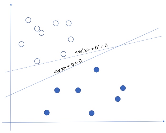
For Support Vector Machine, the goal is to find a decision boundary (line/hyperplane) such that the distance from the decision boundary to each support vectors are equal.
The SVM is also called Max-Margin Classfier, because its objective is to maximize the distance between support vectors and decision boundary.
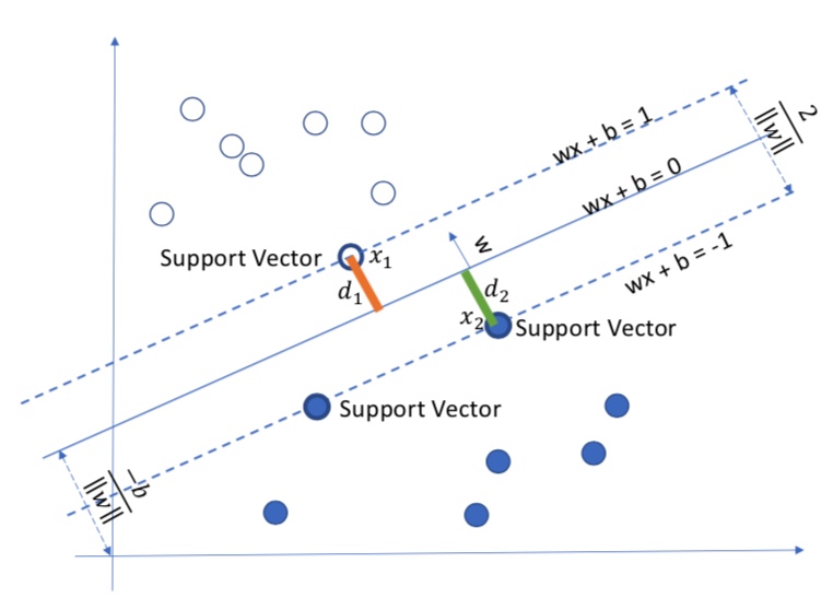
Let $x_1, x_2$ be the support vectors of their corresponding class, their distance to the boundary $w^Tx+b=0$ is $d_1$, $d_2$.
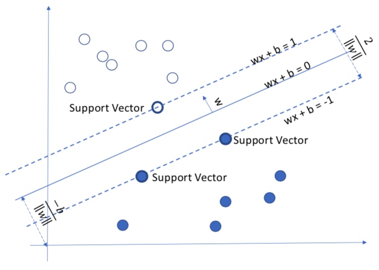
$w$ is a vector which is perpendicular to the decision line. The support vectors are the data point in a class who are closest to the boundary. It is obvious that we have:
\[w^Tx_1 + b = 1\\ w^Tx_2 + b = -1\]The 1 and -1 is the label of the class, the vanilla SVM handles the binary classification problem so the class label is either 1 or -1.
Now we do some transformation on the above equation sets:
\[(w^Tx_1 + b) - (w^Tx_2 + b) = 2\\ w^T(x_1-x_2) = 2 \\ w^T(x_1 - x_2) = \|w\|_2\|x_1-x_2\|_2cos\theta=2 \\ \|x_1-x_2\|_2cos\theta = \frac{2}{\|w\|_2} \\\]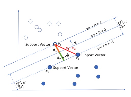
From the figure illustration, we can see that this is equals to the distance between two support vector, i.e.:
\[d_1 + d_2 = \|x_1-x_2\|_2cos\theta = \frac{2}{\|w\|_2} \\\]2. Mathematical Model of SVM
2.1 The original SVM and its dual problem
The goal of SVM is to maximize the margin, i.e. maximize $d_1+d_2 = \frac{2}{|w|_2}$. This can be converted to a minimization problem where we want to minimize the demoninator$|w|_2$. Thus, the Support Vector Machine is formulated as:
\[\begin{align} \min_{w,b} \ \ & \frac{1}{2}\|w\|^2 \\ s.t. \ \ & y_i ( w^T x_i + b)\ge1, i=1,...,n \end{align}\]The constraint requires that all data points should be classify to their corresponding classes.
Now we will try to solve this optimization problem using Lagrangian. We fisrt rewrite constraint as:
\[g_i(w) = -y_i(w^Tx_i + b) + 1 \le 0\]Based on Lagrangian, the problem can be formulated as:
\[\mathcal{L}(w, b, \alpha) = \frac{1}{2}\|w\|^2 - \sum^n_{i=1}\alpha_i [y_i(w^Tx_i + b) - 1]\]The object function becomes:
\[\min_{w,b}\max_{\alpha_i\ge 0}\mathcal{L}(w,b,a)=p^*\]This objective is not easy to solve as we are dealing with two parameters and $\alpha_i$ are inequality constraint. So we consider its dual form:
\[\max_{\alpha_i\ge 0}\min_{w,b} \mathcal{L}(w,b,a)=d^*\]According to the weak duality, $d^*\le p^*$. Also, once the support vector is given, any data point above/below the support vector is a strictly feasible solution. According to the Slater’s condition, the strong duality holds, i.e. $p^*=d^*$. Hence, solving the dual problem leads to the same optimal solution of the original problem.
2.2 Solving the dual problem
We first solve the inner minimization problem. Based on the fact that the derivative of $\mathcal{L}$ w.r.t. to $w$ and $b$ is 0 at the optimal point. We start by calculating the derivative of $\mathcal{L}$ w.r.t. $w$ and $b$.
\[\begin{align} \nabla_w\mathcal{L}(w,b, \alpha) & = \frac{1}{2}\nabla_w\|w\|^2 - \sum^n_{i=1}\alpha_i \nabla_w[y_i(w^Tx_i + b) - 1] \\ & = w - \sum^n_{i=1}\alpha_i y_i x_i \\ \end{align}\]Since $\nabla_w\mathcal{L}(w,b, \alpha) = 0$, we have:
\[w - \sum^n_{i=1}\alpha_i y_i x_i = 0 \implies w = \sum^n_{i=1}\alpha_i y_i x_i\]The derivative w.r.t. to $b$ is:
\[\begin{align} \nabla_b\mathcal{L}(w,b, \alpha) & = - \sum^n_{i=1}\alpha_i \nabla_b[y_i(w^Tx_i + b) - 1] \\ & = - \sum^n_{i=1}\alpha_i y_i\\ \end{align}\] \[-\sum^n_{i=1}\alpha_i y_i = 0 \implies \sum^n_{i=1}\alpha_i y_i = 0\]By substituting $w$ to the Lagrangian we have:
\[\mathcal{L}(w, b, \alpha) = \sum^n_{i=1}\alpha_i - \frac{1}{2}\sum^{n}_{i, j=1}\alpha_i \alpha_j y_i y_j x_i^T x_j\]The deduction is a little bit complicated, click below to see step-by-step deduction.
Step-by-step Deduction
$$ \begin{align} \mathcal{L}(w, b, \alpha) & = \frac{1}{2}\|w\|^2 - \sum^n_{i=1}\alpha_i [y_i(w^Tx_i + b) - 1] \\ & = \frac{1}{2}w^Tw - \sum^n_{i=1}\alpha_iy_iw^Tx_i - \sum^n_{i=1}\alpha_i y_i b + \sum^n_{i=1}\alpha_i \\ & = \frac{1}{2}w^T\sum^n_{i=1}\alpha_i y_i x_i - w^T\sum^n_{i=1}\alpha_i y_i x_i - \sum^n_{i=1}\alpha_i y_i b + \sum^n_{i=1}\alpha_i \\ & = -\frac{1}{2}w^T\sum^n_{i=1}\alpha_i y_i x_i - \sum^n_{i=1}\alpha_i y_i b + \sum^n_{i=1}\alpha_i \\ & = -\frac{1}{2}\sum^n_{i=1}(\alpha_i y_i x_i)^T\sum^n_{i=1}\alpha_i y_i x_i - \sum^n_{i=1}\alpha_i y_i b + \sum^n_{i=1}\alpha_i \\ & = -\frac{1}{2}\sum^n_{i=1}\alpha_i y_i x_i^T\sum^n_{i=1}\alpha_i y_i x_i - \sum^n_{i=1}\alpha_i y_i b + \sum^n_{i=1}\alpha_i \\ & = -\frac{1}{2}\sum^n_{i, j=1}\alpha_i y_i x_i^T\alpha_j y_j x_j - \sum^n_{i=1}\alpha_i y_i b + \sum^n_{i=1}\alpha_i \\ & = \sum^n_{i=1}\alpha_i - \frac{1}{2}\sum^n_{i, j=1}\alpha_i \alpha_j y_i y_j x_i^T x_j \end{align} $$
Now the Lagrangian only includes a single parameters $\alpha$. Solving the optimal $\alpha$ reveals the optimal $w$ and $b$. Thus, the optimization problem becomes:
\[\begin{align} \max_a \ \ &\sum^n_{i=1}\alpha_i - \frac{1}{2}\sum^n_{i, j=1}\alpha_i \alpha_j y_i y_j x_i^T x_j \\ s.t. \ \ &\alpha_i \ge 0, i = 1,...,n \\ & \sum^n_{i=1}\alpha_i y_i = 0 \end{align}\]Once we get the optimal $\alpha^*$, we can get $w^*$ by the fact that $w = \sum^n_{i=1}\alpha_i y_i x_i$.
Then we can get $b^*$ by
\[b^* = -\frac{max_{i:y_i=-1}w^*Tx_i + min_{i:y_i=1}w^*Tx_i}{2}\]The Lagrange multiplier $\alpha$ can be solved by SMO algorithm.
2.3 Classification with SVM
Once we solved the optimization problem and obtained the SVM parameters, we can use it to classify new data point. Given a data point $x$, the decision is made by the sign of the following:
\[\begin{align} w^Tx + b & = (\sum^n_{i=1}\alpha_i y_i x_i)^Tx + b \\ & = \sum^n_{i=1}\alpha_i y_i x_i^Tx + b \\ & = \sum^n_{i=1}\alpha_i y_i <x_i, x> + b \end{align}\]where $<a,b>$ is the inner product between vector $a$ and vector $b$.
One may think that this computation is expensive, as given a new data point, we need to calculate the inner product between $x$ and every training data. If we have 1 billions of training data, this process will take a while to finish. However, the design of SVM actually utilizes a very beautiful property: remember that the strong duality holds for SVM? This implies that KKT condition also holds as it is a necessary condition for strong duality.
The KKT condition includes Complementary Slackness ($\alpha^*g_i(w^*)=0$) which says:
\[\begin{cases} \alpha_i^*=0, \ \ g_i(w^*)<0 \\ \alpha_i^*\gt0, \ \ g_i(w^*)=0 \end{cases}\]We can see that, when $g_i(w) = -y_i(w^Tx_i + b) + 1 \le 0$, the Lagrange multiplier $\alpha=0$. This means that only the support vectors has the actual influence in the final decision process. Thus, we only need to calculate the inner products between new data point and support vectors.
3. SVM With Slack Variable
3.1 Outlier
In the real-world application scenario, sometimes we have some noisy data point that locates in an unusual position which we call them outliers.
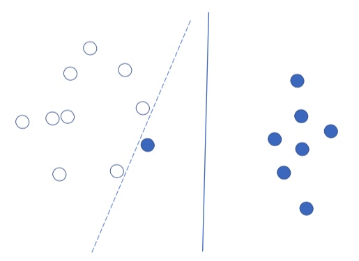
Solving the original problem for all data point including these outliers may have negative influence to the learned model. In the figure above, there is a blue point that locates in an unusual location, and the original SVM will shift its decision boundary to the left because of this outlier.
A worst case is that if this blue point is located in the center of white points, then we will not be able to find a hyperplane to separate these two classes.
3.2 Slack variable
To handle this problem, we will modify the original problem such that we allow the data point can be off the center within a certain distance.
\[\begin{align} \min_{w,b} \ \ & \frac{1}{2}\|w\|^2 + C\sum_{i=1}^n \xi_i \\ s.t. \ \ & y_i ( w^T x_i + b)\ge1-\xi_i, \ i=1,...,n \\ &\xi_i \ge 0, i = 1,...n \end{align}\]The dual problem:
\[\begin{align} \max_a \ \ &\sum^n_{i=1}\alpha_i - \frac{1}{2}\sum^n_{i, j=1}\alpha_i \alpha_j y_i y_j x_i^T x_j \\ s.t. \ \ & 0\le \alpha_i \le C, \ i = 1,...,n \\ & \sum^n_{i=1}\alpha_i y_i = 0 \end{align}\]We can see that for the dual problem, the only difference is that the constraint for $\alpha_i$ now has an upper bound $C$.
Also the Complementary Slackness in the KKT condition becomes:
\[\begin{cases} \begin{align} \alpha_i^*=0, \ \ &y_i ( w^T x_i + b) \gt 1 \\ \alpha_i^*=C, \ \ &y_i ( w^T x_i + b) \lt 1 \\ 0 \lt \alpha_i^*\lt C, \ \ &y_i ( w^T x_i + b) = 1 \end{align} \end{cases}\]3.2.1 Extension: Hinge Loss and SVM
Consider a Support Vector Machine with slack variables, it’s constraints is:
\[y_i ( w^T x_i + b)\ge 1-\xi_i \implies \xi_i \ge 1 - y_i ( w^T x_i + b) \\ \xi_i \ge 0\]Which can be summarized as:
\[\xi_i = max(0, 1 - y_i ( w^T x_i + b))\]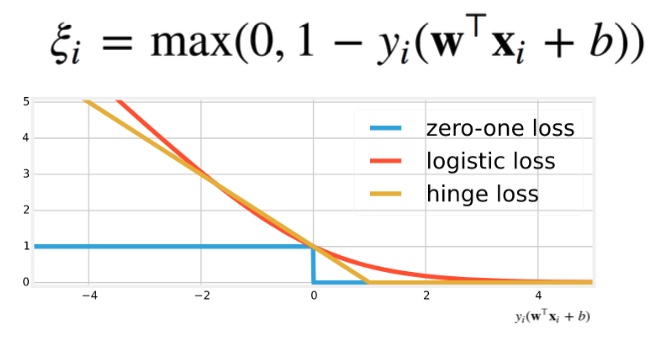
Hinge loss is wildly used in neural networks as it can be optimized by gradient descent. Optimizing Hinge loss has the same effect as SVM.
- Hinge Loss is convex.
- The gradient when $x<0$ is small, so it has fewer penalty to wrong classification.
- The loss is 0 when $x\ge 1$, i.e. if a classifiction is correct with enough confidence, then it will stop optimizing for this data.
- Not differentiable when $x=0$, need to do piecewise derivation.