Machine Learning Note: Support Vector Machine (2)
06 March 2020
4. Kernel SVM
4.1 Kernel Trick
Recall the dual form of the SVM problem:
\[\begin{align} \max_a \ \ &\sum^n_{i=1}\alpha_i - \frac{1}{2}\sum^n_{i, j=1}\alpha_i \alpha_j y_i y_j x_i^T x_j \\ s.t. \ \ &\alpha_i \ge 0, i = 1,...,n \\ & \sum^n_{i=1}\alpha_i y_i = 0 \end{align}\]We could have some intuitive interpretation of this form:
- $x_i^T x_j$ measures the similarity of two data point by inner product.
- $y_iy_j$ is positive if two data points are in the same class, and is negative if they belong two different classes.
- $\alpha$ control the importance of different data points, and $\sum^n_{i=1}\alpha_i y_i = 0$ makes sure that the total weights of two different classes are equal.
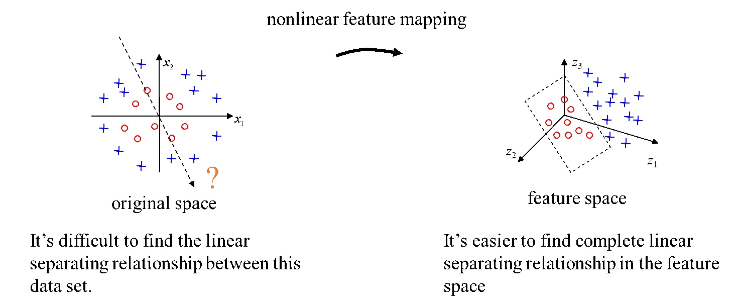
Notice that we currently use the inner product to measure the similarity between two data points, but the data points are not always linear separable. To solve this proble, we can use a kernel to map these data points to a high dimensional space where the converted points can be separated.
\[\begin{align} \max_a \ \ &\sum^n_{i=1}\alpha_i - \frac{1}{2}\sum^n_{i, j=1}\alpha_i \alpha_j y_i y_j K(x_i^T x_j) \\ s.t. \ \ &\alpha_i \ge 0, i = 1,...,n \\ & \sum^n_{i=1}\alpha_i y_i = 0 \end{align}\]Where $K(x_i, x_j) = \langle \Phi(x_i), \Phi(x_j) \rangle$
Notice that we didin’t change any other part of the function but replace $x^T_ix_j$ with $K(x_i, x_j)$.
Intuitively, kernel functions map the data point to a high dimensional space (also called Hilbert Space) before calculating the inner product.
4.2 Mercer’s condition
In this context, a kernel is define as a symmetric mapping function which maps $R^n \times R^n \to R$. Where symmetric means that $K(x, y)=K(y, x)$
If a function returns the inner products of two input in another space, i.e. $K(x, y) = \langle \Phi(x), \Phi(y) \rangle$, then this $K(x, y)$ is a kernel.
However, how do we know if a kernel satisfy this property? The answer is given by Mercer’s condition (here I use the definition from this link).
Theorem (Mercer’s Condition). There exists a mapping $\Phi$ and an expansion:
\[K(x, y) = \langle \Phi(x), \Phi(y) \rangle\]if and only if, for any $g(x)$ such that:
\[\int g(x)^2dx \text{ is finite}\]then
\[\int K(x, y)g(x)g(y)dxdy\ge0.\]However, the above case is hard to check as we need to check for all $g$ with finite $L_2$ norm. However, the condition is satisfied if the Kernel Matrix is positive semi-definite
Also check here for some proof of this theorem.
The Mercer’s condition basically tells that if a kernel can be expressed as a inner product in a Hilbert Space. This is very useful as sometimes we don’t explicitly know the mapping function $\Phi$ (they might be very complicated to express), but we can know if $\Phi$ and the corresponding Hilber Space $\mathcal{H}$ exists by checking this condition.
4.3 Common Kernels
Polynomial Kernel
\[\begin{align} K(x_i, x_j) = (\langle x_i, x_j\rangle + c)^d \end{align}\]$c \geq 0 $ controls the intensity of low-rank terms.
When $c=0, d=1$, the polynomial kernel becomes linear kernel, which equals to the SVM without any kernel.
\[\begin{align} K(x_i, x_j) = \langle x_i, x_j \rangle \end{align}\]Example:
$x_i = [x_{i1}, x_{i2}]$ $x_j = [x_{j1}, x_{j2}]$
Consider a polynomial kernel function:
\[\begin{align} K(x_i, x_j) & = \langle x_i, x_j \rangle^2 (c=0, d=2) \\ & = (x_{i1}x_{j1} + x_{i2}x_{j2}) ^ 2 \\ & = (x_{i1}^2x_{j1}^2 + x_{i2}^2x_{j2}^2 + 2x_{i1}x_{i2}x_{j1}x_{j2}) \\ & = \langle \Phi(x_i), \Phi(x_j) \rangle \end{align}\]The above kernel can be explicitly represented as:
\[\begin{align} \Phi(x_i)= [x_{i1}^2, x_{i2}^2, \sqrt2x_{i1}x_{i2}] \\ \Phi(x_j)= [x_{j1}^2, x_{j2}^2, \sqrt2x_{j1}x_{j2}] \end{align}\]We can see that the polynomial kernel in this example map the original 2-dimension vectors into a new 3-dimension space.
Gaussian Kernel (also called Radial Basis Function (RBF) Kernel)
\[\begin{align} K(x_i, x_j) = exp(-\frac{||x_i-x_j||^2_2}{2\sigma^2}) \end{align}\]$\sigma$ is a hyper-parameters.
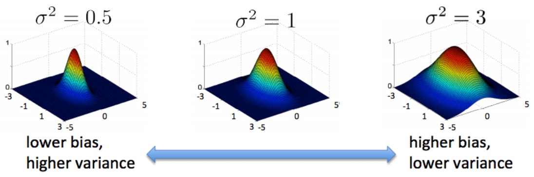
- When $x_i=x_j$, $K(x_i, x_j) = 0$.
- When distance between $x_i$ and $x_j$ increases, $K(x_i, x_j)$ heads to 0.
- To use gaussian kernel we need to normalize the features (e.g. -mean/std).
Sigmoid Kernel
\[\begin{align} K(x_i, x_j) = tanh(\alpha x_i^Tx_j + c) \end{align}\]With this kernel, the SVM is equivalent to a neural network without hidden layers.
Cosine Similarity
\[\begin{align} K(x_i, x_j) = \frac{x_i^Tx_j}{||x_i||||x_j||} \end{align}\]- Measures the cosine similarity of two vectors
5. Solving SVM
SVM is a QP problem which can be solved within polynomial times.
Coordinate Descent
- Search 1 single variables during each iteration and fix all the other variables.
- Convert the multi-dimensions optimization problem into a single-dimension optimization problem. Thus it is called coordinate descent.
During each iteration:
\[\begin{align} x_i^{(k)} &= x_{i-1}^{(k)} + \alpha_i^{(k)}d_i^{(k)} \\ d_i^{(k)} &= e_i\\ k&=0,1,2,...\\\ i&=1,2,...,n \end{align}\]Convergence Criterion:
\[\begin{align} ||x_n^{(k)} - x_0^{(k)}|| \leq \epsilon \\ x^* \leftarrow x_n^{(k)} \end{align}\]Sequantial minimal optimization (SMO)
Recall the SVM with slack variables (dual form):
\[\begin{align} \max_a \ \ &\sum^n_{i=1}\alpha_i - \frac{1}{2}\sum^n_{i, j=1}\alpha_i \alpha_j y_i y_j x_i^T x_j \\ s.t. \ \ & 0\le \alpha_i \le C, \ i = 1,...,n \\ & \sum^n_{i=1}\alpha_i y_i = 0 \end{align}\]also KKT Conditions:
\[\begin{cases} \begin{align} \alpha_i^*=0, \ \ &y_i ( w^T x_i + b) \gt 1 \\ \alpha_i^*=C, \ \ &y_i ( w^T x_i + b) \lt 1 \\ 0 \lt \alpha_i^*\lt C, \ \ &y_i ( w^T x_i + b) = 1 \end{align} \end{cases}\]the set of $\alpha_i$ that satisfies KKT Condition is the solution of the SVM.
We could solve this SVM using the following SMO algorithm:
Repeat Until Converge{
- Select the $\alpha_i$ and $\alpha_j$ to optimize in this step.
- Keep other $\alpha_{k\neq i,j}$ unchanged, and only optimize $W(\alpha)$ by only changing $\alpha_i$ and $\alpha_j$.
}
Use KKT Condition as the convergence criterion.
As we can see, the SMO algorithm is a special case of coordinate descent, but in SMO we choose to optimize two variables in each step.
Why use two variables? Becase there is a constrain in the SVM formulation that $\sum^n_{i=1}\alpha_i y_i = 0$. In this case, if we only optimize one variable in a step, any change will violate this constraint.
For more details and implementation of SMO refer to: http://cs229.stanford.edu/materials/smo.pdf
6. SVM for Multi-classes
The vanilla SVM only supports binary classification. Currently there are two methods to apply SVM to multi-class classifications.
- OVR (One Versus Rest): for $K$ classes, we train $k$ SVMs. The $j^{th}$ SVM is used to classify if a data belongs to class $j$ or not. During prediction, the data is classified as class $j$ if $w_j^Tx + b_j$ gives the maximum value.
- OVO (One Versus One): for $K$ classse, we train $C_K^2 = K(K-1)/2$ SVMs. Each SVM only decide if a data belongs to two specific classes that this SVM was trained on. During prediction, $K(K-1)/2$ predictions has been made for each data, and the finally classification is based on voting scores.
7. Conclusions
- SVM is a max-margin classifier, it is not easy to overfit because it only finds one optimal decision boundary.
- Kernel tricks can help SVM to deal with situations when data points are not linearly separable.
Advantages:
- Solid theoratical supports. Convex problem, converged to global optimal.
- Support different kernel functions which gives more flexibities.
Disadvantages
- Could be slow when dataset is large.